What Exactly Are We Estimating When We Talk About ‘Causal Effects’?

When we ask the question “What is the causal effect of X on Y”, it might sound simple. But in reality, this question is quite broad and vague. In causal inference, there is no such thing as the causal effect. Instead, there are several different ‘types’ of causal effects we might be interested in, depending on the context and the goal of our analysis. So when we do causal inference, the first step is to get clear on which specific causal quantity we’re trying to estimate.

In this blog post, I’ll go through some of the most common causal quantities and explain how they differ. These include the individual treatment effect, the conditional average treatment effect, and the average treatment effect.

Individual Treatment Effect

The most fundamental way to define a causal effect is at the individual level. This is called the Individual Treatment Effect (ITE). It refers to the causal effect of a treatment on the outcome for one specific unit.

In this context, treatment means any variable that we are thinking about changing or intervening on. This could be something like whether someone receives a marketing email, takes a medication, gets assigned a new pricing plan, or uses a new feature in a product.

The outcome is the variable we want to measure the effect on. This could be sales, test scores, website clicks, blood pressure, or customer retention, basically anything we care about as a result.

The unit is the entity being studied. This can for example be a person, a store, a household, a company, a country, and so on.

The ITE then captures how the outcome for one specific unit would change if we were to change the treatment. It’s about comparing two possible outcomes for the same unit: one where they receive the treatment, and one where they don’t (in the binary treatment case).

Let’s look at an example.

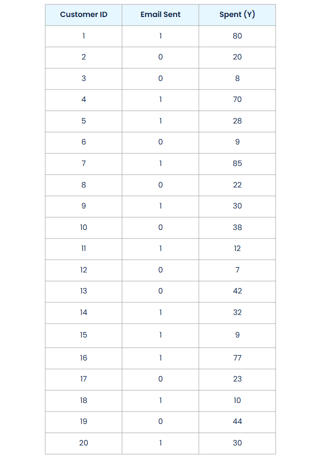
Suppose an e-commerce store ran a promotional email campaign and later measured how much each customer spent in the weeks that followed. For each customer, they collected data on three things: a customer ID, whether or not the customer received the promotional email (1 if yes, 0 if no), and the amount they spent during that period (we’ll call this outcome Y).

In this case, the ITE of sending an e-mail on spending asks:

What is the effect of sending a promotional email on the spending of customer i?

In other words, it aims to compare the amount a customer would spend if they received the email, versus what they would spend if they didn’t.

The problem is, in real life, we only see one of those outcomes, as you can see in the data. Either the customer received the email or they didn’t, and we only observe the outcome under that one condition.

For example, customer 4 received the email and spent 70 dollars. We can write this as Y₄(1) = 70, which represents the outcome for customer 4 under treatment equal to 1. Customer 2 did not receive the email and spent 20 dollars. So we have Y₂(0) = 20, meaning the outcome for customer 2 under treatment equal to 0.

But we don’t observe what customer 4 would have spent without the email — Y₄(0) is missing. And we don’t observe what customer 2 would have spent with the email — Y₂(1) is missing.

This is the core challenge in causal inference: we never get to see both outcomes for the same unit. One of them is always missing. This is often called the fundamental problem of causal inference.

But to introduce the causal quantities of interest, imagine for a moment that we could observe both outcomes. Imagine we had two parallel worlds: in one, each customer received the email, and in the other, no one did. We could then observe both Y(0) and Y(1) for each customer. Suppose the data looked like this:

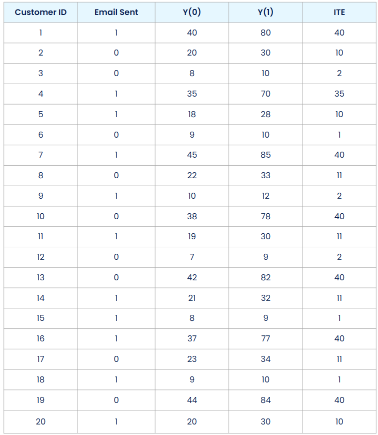
Here, Y(0) is the spending we’d see if the customer didn’t get the email, and Y(1) is the spending if they did. The ITE is then simply the difference between these two outcomes: ITEᵢ = Yᵢ(1) — Yᵢ(0).

For our dataset, the ITE’s are displayed in the right-most column. Each ITE tells us how much the email affected the spending behavior of one specific customer.

We also see how much this ITE varies among customers. Some customers (like customer 1) responded strongly to the email, spending 40 dollars more. Others (like customer 18) showed only a minor increase. This variation in ITE makes sense. People are different, and not everyone reacts the same way to a promotional email.

Okay, so that’s the ITE. Now let’s move on to another quantity: the average treatment effect.

The Average Treatment Effect

The Average Treatment Effect, or ATE, refers to the average causal effect across a population of units. While the ITE looks at individual units, the ATE focuses on what happens on average when we apply a treatment to a group.

More specifically, the ATE is defined as:

ATE = E[Y(1)] – E[Y(0)]

This means: the average outcome we would observe if everyone in the population received the treatment, minus the average outcome we would observe if no one received the treatment.

In our example, let’s say the population is the group of 20 customers. So the ATE tells us the difference in average monthly spending if we had sent the promotional email to all customers, compared to if we had sent it to none.

Let’s go back to our data. Suppose we again in some magical way had access to both spending amounts under treatment (email sent) and spending under no treatment (no email) for each customer.

Then we could compute:

E[Y(0)] = (40 + 20 + 8 + 35 + 18 + 9 + 45 + 22 + 10 + 38 + 19 + 7 + 42 + 21 + 8 + 37 + 23 + 9 + 44 + 20) / 20 = 23.75

E[Y(1)] = (80 + 30 + 10 + 70 + 28 + 10 + 85 + 33 + 12 + 78 + 30 + 9 + 82 + 32 + 9 + 77 + 34 + 10 + 84 + 30) / 20 = 41.65

So the ATE is:

ATE = 41.65 – 23.75 = 17.9

This means that if we had sent the promotional email to every customer in this group, we would expect an increase of 17.9 dollars in monthly spending on average, compared to sending no email at all.

In other words, if we picked a customer at random from this population, our best guess for the effect of the email on their spending would be 17.9 dollars.

We can also see that the ATE is just the average of all the individual treatment effects. So the ATE essentially averages out all the individual differences. This makes it a simpler metric, but also less detailed. It doesn’t tell us how different customers respond to the treatment, it just gives us the overall effect.

This can be a limitation. For example, say that the email would have had a positive effect for some customers and an equally negative effect for others. In such cases, the ATE might be close to zero. But that doesn’t mean the email had no impact — it just means the effects canceled each other out on average. If we could identify which customers respond positively, we could still gain a lot by targeting only them.

This brings us to a more informative metric that sits ‘between’ the ITE and the ATE: the Conditional Average Treatment Effect.

The Conditional Average Treatment Effect

The Conditional Average Treatment Effect, or CATE, is similar to the ATE, but instead of looking at the whole population, we look at subpopulations of units that share certain characteristics. In other words, while the ATE tells us the average treatment effect across all units, the CATE tells us the average effect for a specific subgroups of units.

Formally, we define it as:

CATE(X = x) = E[Y(1) | X = x] — E[Y(0) | X = x]

This means the CATE for units with characteristics X = x is the average outcome we would observe under treatment for that group, minus the average outcome we would observe under no treatment for the same group. The variable X can represent any feature or set of features that we think might influence how the treatment affects the outcome. These could be things like age, gender, location, store size, household size and so on.

Let’s go back to our promotional email example.

We saw earlier that customers respond differently to the email, and we might suspect that some characteristic helps explain why. Suppose we believe that engagement level plays a role. It seems reasonable to assume that highly engaged customers may respond more positively to a promotional email than customers who rarely interact with the store.

To explore this, we add an “engagement score” to our dataset. Each customer is labeled as having low, medium, or high engagement. This score could be based on metrics like website activity, purchase frequency and so on.

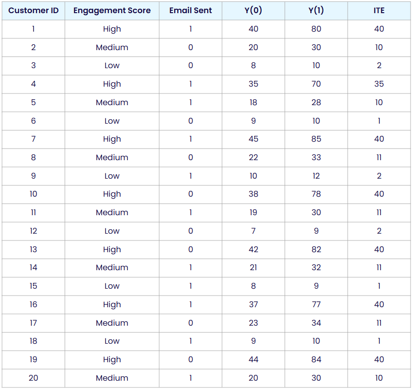
Now we can compute the average treatment effect separately within each engagement group.

First, for customers with low engagement:

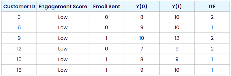
E[Y(1) | engagement = low] = (10 + 10 + 12 + 9 + 9 + 10) /6 = 10
E[Y(0) | engagement = low] = (8 + 9 + 10 + 7 + 8 + 9) / 6 = 8.5
So the CATE for this group is 10–8.5 = 1.5

Next, for customers with medium engagement:

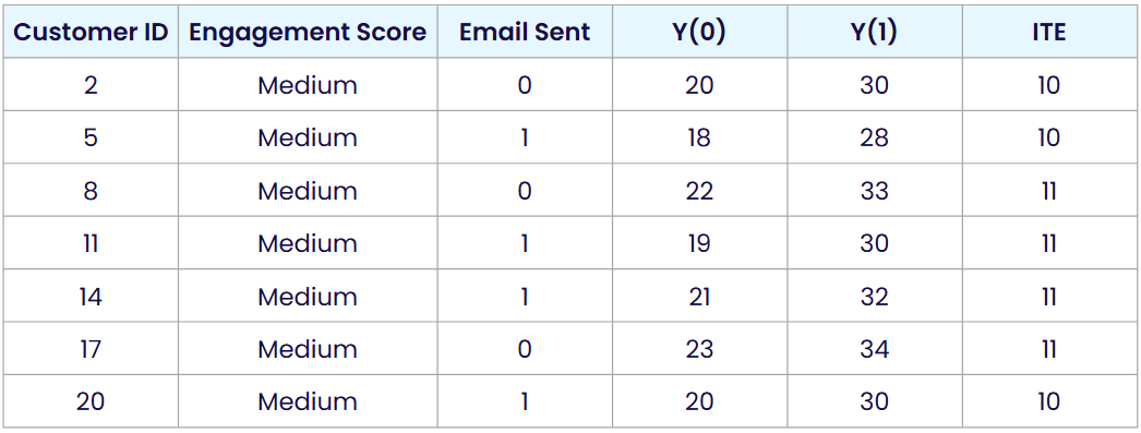
E[Y(1) | engagement = medium] = (30 + 28 + 33 + 30 + 32 + 34 + 30) / 7 = 31
E[Y(0) | engagement = medium] = (20 + 18 + 22 + 19 + 21 + 23 + 20) / 7 ≈ 20.43
So the CATE here is 31–20.43 ≈ 10.57

Finally, for customers with high engagement:

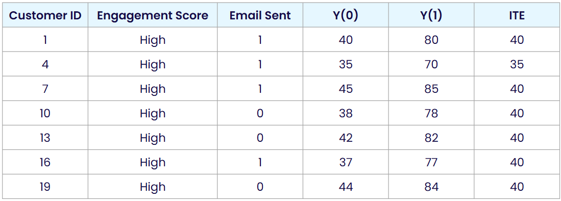
E[Y(1) | engagement = high] = (80 + 70 + 85 + 78 + 82 + 77 + 84) / 7 ≈ 79.43
E[Y(0) | engagement = high] = (40 + 35 + 45 + 38 + 42 + 37 + 44) / 7 ≈ 40.14
So the CATE for this group is 79.43–40.14 ≈ 39.29

To summarize these results:

CATE for low engagement = 1.5
CATE for medium engagement ≈ 10.57
CATE for high engagement ≈ 39.29

We know see that the effect of sending an e-mail is higher for high-engaging customers compared to low-engaging customers.

This kind of information can be especially useful in practice. For example, if sending emails costs money or if we are running a discount campaign where budget is limited, it makes sense to target the customers who are most likely to respond positively. Or if we would see (or in practice estimate) that the effect of the treatment would be harmful for some customers (e.g. reduces their spending), we could decide to exclude them entirely from the campaign.

So in short, moving from ATE to CATE gives us a more personalized view. It helps us make better decisions by focusing on how different groups respond differently to the same treatment.

Causal Inference as a Missing Data Problem

Okay, so those are the main causal quantities we are interested in with Causal Inference in practice. But while I introduced them using outcomes of units under various treatment conditions, this of course doesn’t work in practice. In our example, the data in practice would look like this:

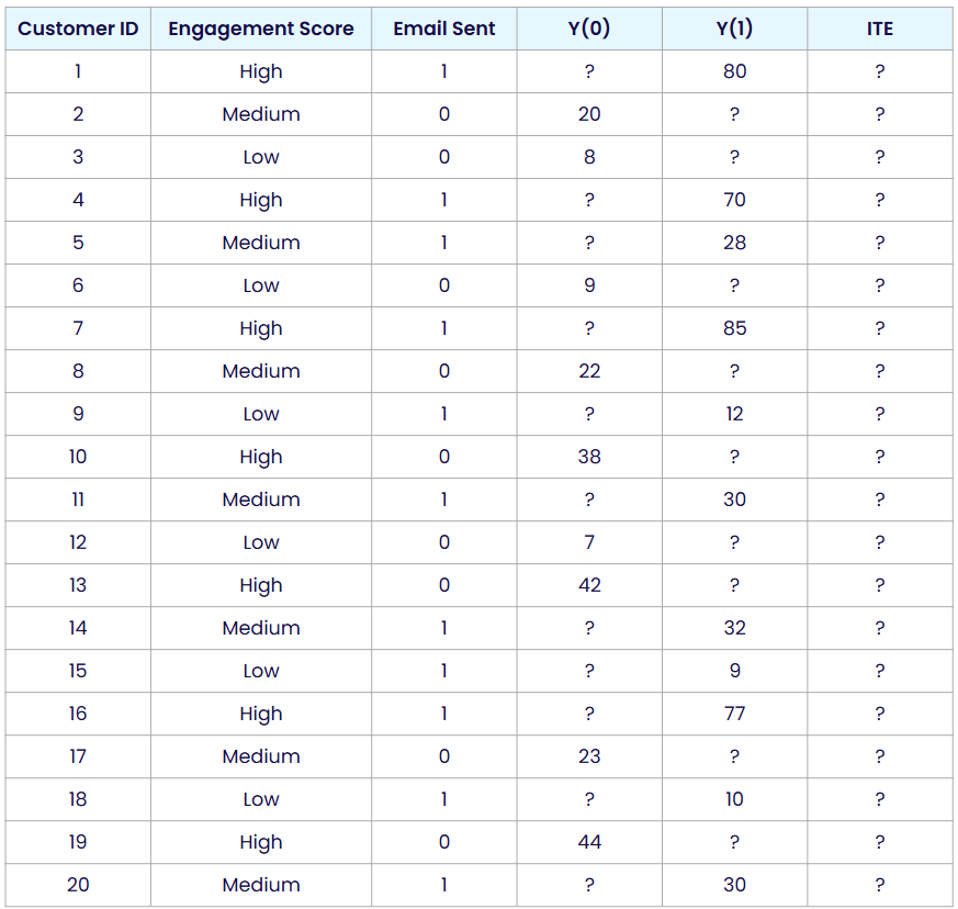
Here we have question marks in all the places where we don’t observe an outcome. For every customer, we only see the outcome under the treatment they actually received. If a customer received the promotional email, we observe how much they spent with the email, but we do not know how much they would have spent without it. And for customers who did not receive the email, we are missing the outcome under treatment. This is the fundamental problem of causal inference I pointed out at the start of this blog post.

This is also why causal inference is often described as a missing data problem. For every unit, we are missing one of the two outcomes we would need to calculate an ITE. A large part of causal inference in practice is then about finding good ways to estimate or approximate those missing outcomes.

So how do we do that? Well, by using information from other, similar units.

For example, to estimate what customer 1 would have spent without receiving the email, we might look at customers who are similar to customer 1 but did not receive the email. Their behavior can give us an idea of what the missing outcome might have been.

When estimating group-level quantities like the ATE or the CATE, we compare average outcomes between groups with different treatments. But again, this only gives valid results if the groups are otherwise similar. That is, they should differ only in the treatment they received, not in other important ways.

This is where the idea of comparability becomes important. The more personalized the question we want to ask, the harder it becomes to find truly comparable units.

If we want to estimate the treatment effect for a specific unit, we would need to find others who are almost identical in every relevant way. That is rarely possible in real-world data.

Estimating the ATE or CATE is usually ‘easier’. Because we are averaging over groups of units, we do not need perfect matches for each unit. Instead, we just need the different treatment groups to be similar on average.

From Binary To Continuous Treatments

In this blog post, I focused on binary treatments, such as sending a promotional email or not. But all the concepts discussed (the ITE, ATE, and CATE ) can be naturally extended to continuous treatments as well. In that case, instead of comparing outcomes between treatment equals 0 and treatment equals 1, we look at different treatment levels.

Examples of continuous treatments include the percentage of a discount offered, the number of hours of training provided, or the dosage of a medication. The idea is the same: we want to understand how changes in the treatment level affect the outcome.

However, with continuous treatments, it becomes infeasible to simply compare average outcomes between treatment groups. There are too many possible treatment values, so we can’t neatly group units as we did in the binary case. Instead, we need to rely on models that can estimate the relationship between treatment level and outcome across the full range of values.

And basically in practice, causal inference almost always depends on models, even for binary treatments. This is because we often need to make sure that the units we compare are truly comparable, and we do this by adjusting for many variables that otherwise would produce differences between them. Without using models such processes become infeasible easily.