Understanding the relationship between Correlation and Causation

While most people in the data industry are familiar with the saying “correlation is not causation” , only few truly know how the two actually relate. This lack of knowledge strongly limits the quality of the data models that are being built.

Knowing the difference between correlation and causation should be a core part of any data education, but unfortunately, it isn’t. This is mainly because causality has been misunderstood for a long time. Recent advancements, mainly due to the work of Judea Pearl, have provided us with tools to understand causality and its relation to correlation on a much deeper level. So, how do correlation and causation relate?

Quick note: From now on, I’ll use the term “association” instead of “correlation”. In the phrase “correlation is not causation,” people often use “correlation” to mean any kind of dependence between variables. But technically, correlation only measures linear dependence. Association, however, covers all types of dependencies, making it a more appropriate term for what we’re discussing.

Association is not Causation, but why not?

Conceptually, we have that Association = Causation + Bias. This means that the associations we observe between variables can be causal, non-causal (bias), or a combination of both!

As humans, it’s natural for us to understand that causation leads to association. For example, rain causes people to carry umbrellas, which means rain and people carrying umbrellas often happen together: a positive association.

However, the concept of bias is often where things get blurry. While it seems intuitive that some associations aren’t directly the result of a causal relationship between the variables we’re looking at, people often struggle to pinpoint exactly what bias is.

So, what is this bias? Well, bias can come in different forms and types. We’ll discuss some of the most prominent ones using examples.

Confounding Bias

Consider the following example: we observe that people who smoke a lot tend to have a higher risk of developing lung cancer compared to people who smoke only a little or not at all — this is a positive association. So, is this association causal, non-causal, or both?

Well, the effect of smoking on lung cancer has been studied through causal analysis, and it has been shown that smoking does cause lung cancer. Therefore, we now know that at least some part of the observed association is causal in nature.

But is there another part that is non-causal, that is, bias? This could be the case!

One source of bias could be the jobs people have. To see this, think about how, in general, construction workers often tend to smoke more than office workers. One reason for this could be that construction workers generally work outdoors, where smoking restrictions are minimal. This means they can smoke more freely throughout the day. In contrast, office workers face stricter indoor smoking rules and fewer opportunities to smoke, which might limit their smoking habits.

But here’s the key point: certain construction jobs also expose workers to harmful materials like asbestos, which can cause cancer on their own.

So in this case, job type both increases smoking rates and cancer risk.

This means that the people we observe smoking more have a higher risk of developing cancer compared to those who smoke less — not only because of smoking itself, but also because of the type of work they do!

This part of the positive association we observe is not causal since it does not come from the effect of smoking on lung cancer, and is therefore due to bias. If we were to simply attribute the entire positive association observed between smoking and lung cancer to the causal effect of smoking, we would overestimate the true causal effect.

The bias in the smoking and lung cancer example is called confounding bias, and the type of job people have is what we call a confounder.

Disclaimer: The source of bias mentioned, while possible, is not supported by specific evidence and is used purely for illustrative purposes.

We can visualize the cause-and-effect relationships in this problem as follows:

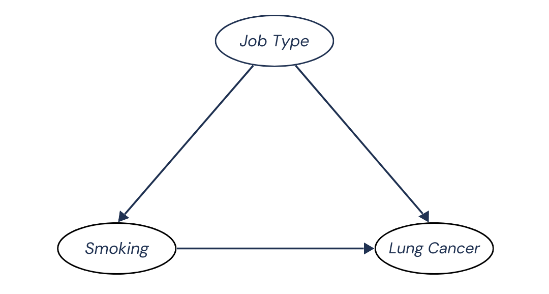
Job Type causes both Smoking and Lung Cancer, and Smoking has a causal effect on Lung Cancer.

This visual is what’s known as a Directed Acyclic Graph (DAG). Judea Pearl popularized the use of this concept to represent the existence of cause-and-effect relationships between variables. In this context, DAGs are also referred to as Causal Graphs.

Removing Confounding Bias

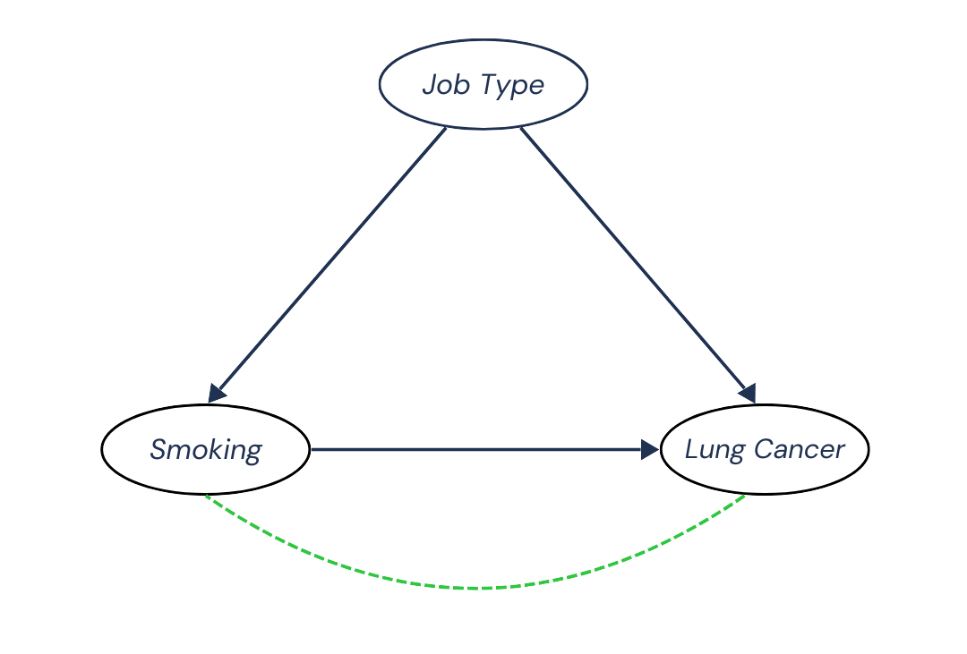
Okay, so Smoking causes Lung Cancer. This means that along the pattern Smoking → Lung Cancer we have a causal dependence, which we also refer to as a causal association. We can represent this dependence with a green dotted line:

At the same time, part of the positive association we observe between Smoking and Lung Cancer is because certain jobs increase both smoking rates and the chances of developing lung cancer. We thus have a non-causal dependence, or non-causal association, along the pattern Smoking ← Job Type → Lung Cancer, represented by a red dotted line:

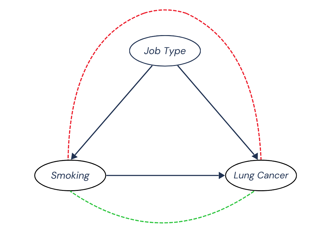
If we want to extract only the causal association from the total association we observe, we need to block this red dependence structure, the bias. How would we do this?

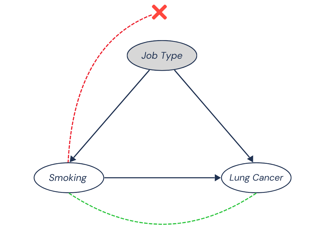
Well, suppose we compare lung cancer rates among people with different smoking rates, but now within groups of people who all have the same job.

In this case, the bias is removed because the bias comes from differences in job types, which affect both smoking habits and cancer risk. Since we no longer have differences in job types, we automatically eliminate this bias.

Thus, by conditioning on the confounding variable (keeping Job Type constant), we remove the confounding bias and we are left only with the causal dependence between smoking and lung cancer!

In this case, association = causation.

Collider Bias

For those a bit more familiar with causality, confounding bias is often the most well-known type of bias. A less commonly known one is called collider bias.

Think about beauty and talent. If you look at the general population, there’s no clear relationship between the two. Some people are both beautiful and talented, some are neither, and some fall somewhere in between. Basically, beauty and talent are independent of each other.

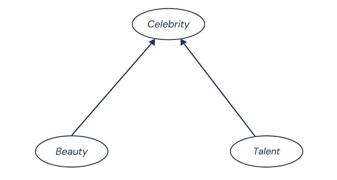
Now, let’s throw a third variable into the mix: being a celebrity or not. Both beauty and talent tend to increase your chances of becoming famous. At the same time, it’s reasonable to assume that there’s no causal relationship between beauty and talent. In other words, becoming more beautiful doesn’t suddenly make you more or less talented, and vice versa.

Our Causal Graph looks like this:

But here’s where things get interesting.

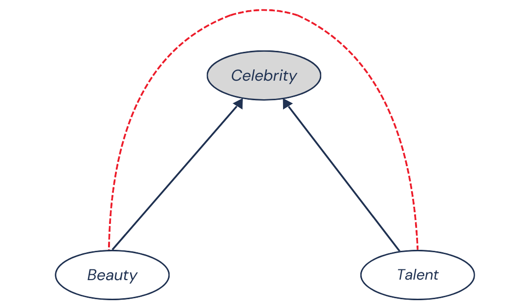
Let’s say we stop looking at the general population and focus only on celebrities. Suddenly, we start seeing a negative association between beauty and talent. Celebrities tend to be either very beautiful or very talented, but not often both. Sure, there are exceptions, but overall, there seems to be a trade-off happening here.

So, conditioning on Celebrity introduces a negative dependence between Beauty and Talent that didn’t exist in the general population. This dependence is non-causal (bias), since it’s not generated by a causal relationship between Beauty and Talent.

Celebrity is called a collider.

Removing Collider Bias

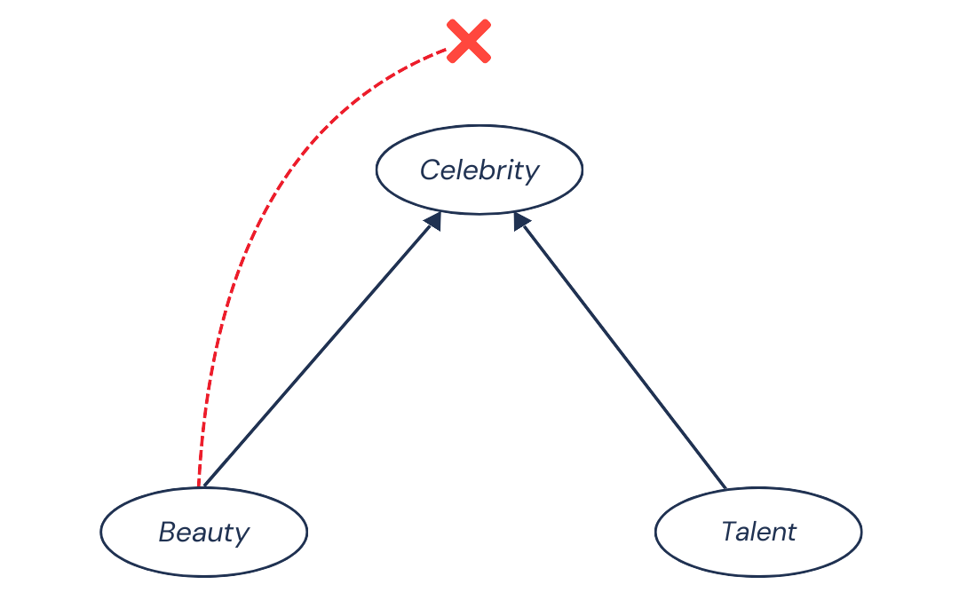
So, we created a non-causal negative association by conditioning on the collider, Celebrity. Without conditioning (looking at beauty and talent in the general population), this bias didn’t exist. So, how to remove this bias? Simple: don’t condition on the collider:

Collider bias is one of the trickiest forms of bias because colliders can often seem like natural choices of variables to include in your model. It might feel like they’re related to the outcome variable and could improve your model. After all, we usually think that adding more variables won’t hurt — the model will sort out what’s important, right?

Well, colliders show us that if you’re doing causal inference, you can’t just throw in any variable. You have to be selective and thoughtful about what you include in your model.

Okay, so you’ve now seen that whereas a confounding variable does harm if we don’t condition on it, a collider variable does harm if we do condition on it!

While collider bias and confounding bias are two major sources of bias, there’s another situation that doesn’t necessarily introduce bias but rather can block out causal dependence structures. This situation is called mediation.

Mediation

Let’s say we have a water leak detection system. The system is designed to detect whether water is leaking, and if it detects a leak, an alarm goes off.

In this scenario, a water leak increases the chances of the detector detecting a leak, which in turn increases the chances of the alarm being triggered.

So, there’s a clear causal effect of water leaking on the alarm going off, but this effect passes through the leak detector. After all, the alarm only goes off if the detector recognizes the leak. Without the detector, the alarm would never go off:

The causal effect of the water leak on the alarm is mediated by the leak detector. The leak detector, in this case, is called the mediator.

So, there is a causal dependence between Water Leak and Leak Alarm, going along the pattern Water Leak → Detect Leak → Leak Alarm:

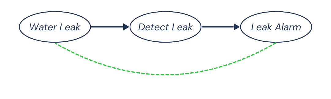
In general, we observe a positive association between Water Leak and Leak Alarm.

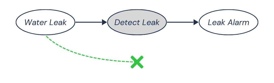
Now, suppose we condition on Detect Leak, meaning we only look at cases where there was a leak detected. Suddenly, Water Leak and Leak Alarm become independent. Why?

Well, the alarm is only triggered when the detector detects a leak. Once the detector detects a leak, whether water is actually leaking becomes irrelevant. Perhaps the detector simply goes off due to a bug! The alarm responds to the detector, not directly to the water leak.

The causal dependence between Water Leak and Leak Alarm is blocked:

Although conditioning on a mediator does not specifically produce “bias”, it does block out a causal dependence structure. Whether this is problematic or not depends on which “type” of causal effect you want to measure.

If you are only measuring the direct effect of Water Leak on Leak Alarm, then you want to remove this indirect causal dependence structure, and so conditioning is necessary.

If you however want to measure the total effect of Water Leak on Leak Alarm, then conditioning would distort the results.

“Just add as many variables as possible”

In practice, conditioning on variables is often done by adding variables to our model. If we are interested in the effect of X on Y, and we include a variable Z in our model, the model will essentially look at how Y varies as X varies, while keeping Z constant.

If Z is a confounding variable, excluding the variable means bias, whereas including the variable removes this bias.

If Z is a collider variable, excluding the variable means no bias, whereas including the variable means bias.

If Z is a mediating variable, excluding the variable means you are also measuring the indirect causal effect of X on Y through Z. Including it removes the indirect effect, meaning you’re no longer measuring the total causal effect of X on Y.

In the era of big data, it’s tempting to think that adding many variables will improve the model. However, now you know that with causal inference, your choice of variables is extremely important, and will determine whether you measure association or causation.