The Role of Seasonality in Causal Inference

Most businesses operate in environments that to some extent change in ‘typical’ ways over time. Customers behave differently around holidays than they do during regular weeks. Traffic on an e-commerce website varies between weekdays and weekends. Purchasing behaviour shifts around paydays, vacation periods, and specific events. These regular fluctuations are all forms of seasonality.

When we perform causal inference, we often work with a fixed period of observational or experimental data. For example, we might analyse the time window from October 1st 2025 to December 1st 2025. Within this window, we estimate the effect of some treatment on an outcome. This could be an experiment in which units are randomly assigned to be exposed to some treatment, or it could be an observational analysis in which units fall into treated and untreated groups in non-randomized ways. In the context of e-commerce, units are often customers.

Because analysis windows often span several weeks, it is common that the data contains multiple seasonal conditions. These conditions can differ in how many customers are active, how likely they are to purchase, how they respond to marketing, and how they interact with a product. It is therefore natural to ask whether these seasonal patterns affect our causal effect estimates, and if so, in what way.

In this blog post, I am going to answer that question, taking a perspective from both observational analyses and experiments.

Let’s start by introducing some notation and causal inference fundamentals.

Notation and Causal Inference Fundamentals

In any causal analysis, we have the following core elements: the treatment, the outcome, and the population of units we study.

I will use T to denote the treatment. This is the variable that we imagine intervening on. For example, T might indicate whether a customer was shown a discount banner, whether they received a basket reminder email, or whether they were exposed to a new ranking algorithm.

I will use Y to denote the outcome, which is the variable whose response to the treatment we want to understand. This might be revenue per customer, whether someone clicked or made a purchase, or the number of items added to a cart.

The population refers to the set of units for which we want to estimate the effect. In many business settings, these units are customers or sessions, but they can also be stores or products for example. The population determines the scope of the effect we are estimating and the group to which our conclusions apply.

To formalise causal effects, it is useful to think in terms of potential outcomes. For each unit i, we imagine two quantities: the outcome the unit would have under treatment, denoted Yi(1), and the outcome the unit would have under no treatment, denoted Yi(0). The causal effect of the treatment for a specific unit is the difference Yi(1) − Yi(0). This quantity is called the Individual Treatment Effect (ITE) for unit i.

The Average Treatment Effect (ATE) is the average of Yi(1) − Yi(0) across all units in the population of interest. So if we take the average of all the ITEs for units in some target group, we obtain the ATE, which reflects how the treatment affects the outcome on average across that group.

We also have Conditional Average Treatment Effects, or CATEs. A CATE is the average of Yi(1) − Yi(0) for units that share a particular characteristic. For example, we can compute the average treatment effect separately for customers with high or low historical engagement. In that case, the characteristic that defines the subgroups is the historical engagement HE, and the CATE for HE = x is the average treatment effect for units whose historical engagement equals x.

Finally, in this blog post, I am going to use the variable S to denote the seasonal condition under which a unit appears in the data. S represents underlying seasonal drivers that can impact how customers or the business behaves. Think of factors such as the number and type of national festivities taking place, positioning relative to typical travel periods, or positioning relative to payday cycles.

How Seasonality Enters the Data

Now that the basic causal quantities and notation are defined, we can start looking at the role that seasonality can play in a causal analysis. The seasonal condition S can be viewed as another (set of) variable(s) in the data-generating process, and its relevance depends on how it interacts with the treatment, the outcome, or both.

Seasonality may influence how likely a unit is to receive the treatment. It may influence what values we typically observe for the outcome. And the magnitude of the treatment effect may differ across seasonal conditions.

Depending on which of these patterns occur in the data-generating process, seasonality can affect causal analysis in different ways. In this blog post, I will focus on two specific roles that S can take: one in which it acts as a common cause of the treatment and the outcome, and one in which the treatment effect varies across seasonal conditions. At the end, I will tie these roles together.

Seasonality as a Common Cause of Treatment and Outcome

Seasonality functions as a common cause when the seasonal condition S affects both the probability of being exposed to the treatment and the outcome Y. This situation appears frequently in observational business data because, in such data, treatment assignment is not random. Instead, it can depend on operational decisions, marketing strategies, and/or customer behaviour that all vary with the seasonal pattern of the business.

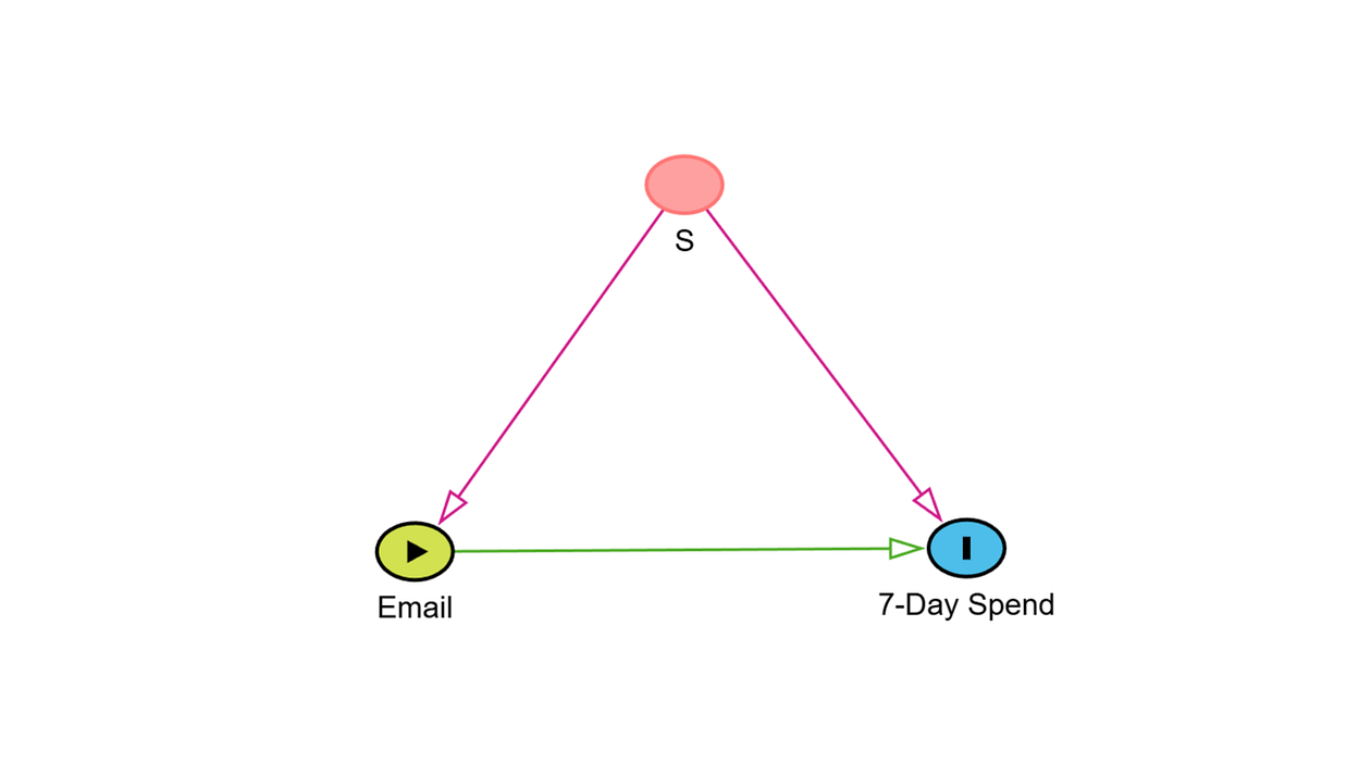
To make this concrete, consider the following example. Suppose we work at an e-commerce company and want to estimate the effect of sending a specific promotional email on customer spending. The treatment T indicates whether a customer received this email. The outcome Y is the amount the customer spends in the week after the email decision was made. The goal is to estimate how receiving this email affects spending in that 7-day period.

Now suppose that the marketing team assigned this email over a period of time, but the probability of sending it was not constant. During high traffic periods, such as the weeks leading up to a major holiday, the team used the campaign more aggressively. For each eligible customer, the probability of receiving the email was higher in these periods. During low traffic periods, the campaign was used more conservatively, and the probability of receiving the email was lower. In this case, the seasonal condition S affects the chances of being exposed to the treatment indirectly through changes in traffic.

Customer spending in the 7-day window also depends on the season. Different seasonal conditions come with systematic differences in how people behave. For example, customers may have stronger purchase intent during periods with many festivities, they may have more disposable income immediately after payday, or they may be preparing for specific events such as holidays. As a result, customers observed under high-season conditions tend to spend more in the same 7-day window than customers observed under low-season conditions.

This would make the seasonal condition S a common cause of sending an email or not (the treatment) and 7-day spend (the outcome), and this will create a problem.

To explain this in a simple way, suppose that we divide the seasonal conditions into two categories. One category represents low-season conditions. These are periods in which the underlying drivers of purchasing behaviour are relatively weak. For example, customers have fewer event-related needs, lower purchasing motivation, or less financial capacity. The other category represents high-season conditions. These are periods in which the underlying drivers of purchasing behaviour are stronger. Customers have clearer reasons to buy, more motivation to browse, and more financial capacity.

If the probability of receiving the email is higher during high-season conditions than during low-season conditions, then the treated group will contain a larger share of customers who happened to be observed in high-season conditions. At the same time, if the email is assigned less frequently during low-season conditions, the untreated group will contain a larger share of customers observed in low-season conditions.

To illustrate this, suppose that during our study window, one third of the customers appeared under low-season conditions and two thirds under high-season conditions. This mimics the idea that high-season periods often generate more traffic, so the number of high-season customers can outweigh the number of low-season customers if the study window includes such periods.

Next, suppose that the probability of receiving the email is 0.4 for customers appearing in low-season conditions and 0.6 for customers appearing in high-season conditions. With large enough sample sizes, this leads to the following proportions:

For low-season customers:
treated: (1/3) × 0.4 = 0.1333
untreated: (1/3) × 0.6 = 0.2000

For high-season customers:
treated: (2/3) × 0.6 = 0.4000
untreated: (2/3) × 0.4 = 0.2667

We can now compute the seasonal composition within each treatment group.

• For the treated group, the total share is 0.1333 + 0.4000 = 0.5333. So:
  low-season share = 0.1333 / 0.5333 ≈ 25%
  high-season share = 0.4000 / 0.5333 ≈ 75%

• For the untreated group, the total share is 0.2000 + 0.2667 = 0.4667. So:
  low-season share = 0.2000 / 0.4667 ≈ 42.9%
  high-season share = 0.2667 / 0.4667 ≈ 57.1%

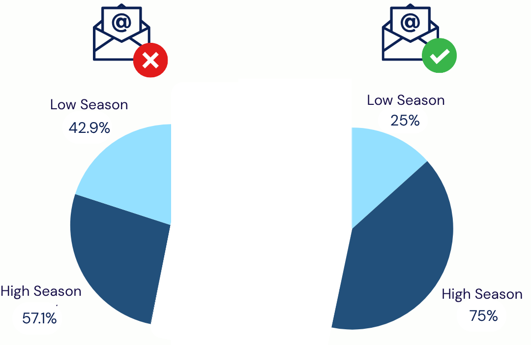
This means that the treated group contains a much larger fraction of high-season customers (75%) than the untreated group (57.1%). The untreated group contains a much larger fraction of low-season customers (42.9%) than the treated group (25%). In other words, the distribution of seasonal conditions S differs between treated and untreated units. These differences arise purely because the probability of receiving the email depends on the seasonal condition. As a result, just comparing the average spend of treated and untreated units will not isolate the causal effect of the email. Part of the difference in average spend might come from the treatment, but part of it will also come from the fact that the two groups were exposed to different seasonal conditions (bias!).

To understand this more clearly, consider what would happen if the email had no effect at all. Because the treated group contains more customers from high-season conditions, it would still show a higher average spend. Because the untreated group contains more customers from low-season conditions, it would still show a lower average spend. The comparison between the two groups would therefore show a positive difference, even though the true effect is zero. This difference is created entirely by the imbalance in seasonal conditions.

ATE ≠ E[Y | T = 1] − E[Y | T = 0].

The way to address this is to compare treated and untreated units under the same seasonal condition. Instead of comparing the full treated group with the full untreated group, we compare treated and untreated customers who were observed in high-season conditions, and we separately compare treated and untreated customers who were observed in low-season conditions. Within each seasonal condition, it can no longer be the case that differences in seasonal conditions produce outcome differences between treated and untreated units, simply because there are no seasonal differences anymore. This allows the comparison to isolate the effect of the email.

This leads to two subgroup effects:

CATE(low season) = E[Y | T = 1, S = low season] − E[Y | T = 0, S = low season]

CATE(high season) = E[Y | T = 1, S = high season] − E[Y | T = 0, S = high season]

These are the average treatment effects for customers who were observed under low-season conditions and high-season conditions, respectively.

If our goal is to recover a single average effect for the entire customer population, we take a weighted average of these two conditional effects. The weights reflect how frequently each seasonal condition occurs in the target population. In our running example, one third of customers appear under low-season conditions and two thirds under high-season conditions. The population ATE is therefore:

ATE = (1/3) × CATE(low season) + (2/3) × CATE(high season).

This weighted average isolates the causal effect of the email because each conditional effect is estimated within a fixed seasonal condition, and the weighting step simply reconstructs the environment of the target population. When seasonality acts as a common cause of T and Y, adjusting for S in this way removes the bias that would otherwise arise from comparing groups with different seasonal compositions.

So, to summarise, the first role seasonality can play in a causal analysis is that it can function as a common cause of the treatment and the outcome. In that case, it produces a biased association between the two, and we cannot simply compare average outcomes to measure causal effects. Adjusting for the seasonal condition resolves this problem.

Let’s now focus on the second scenario, where seasonality does not act as a common cause of treatment and outcome, but the treatment effect differs across seasonal conditions.

When Treatment Effects Differ Across Seasonal Conditions

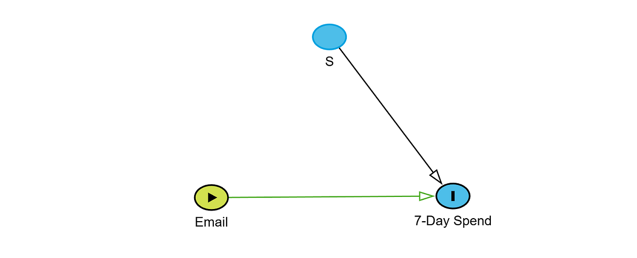
In the observational case we just discussed, the probability of receiving the email depended on the seasonal condition S, which made S a common cause of the treatment and the outcome. In a randomized experiment, this is no longer true. The defining property of randomization is that every unit has the same probability of being exposed to the treatment, independent of the seasonal condition under which the unit appears.

To continue with the same example, suppose we now run a randomized experiment in which every eligible customer is assigned to receive the promotional email with probability 0.5, and to not receive it with probability 0.5. The outcome Y remains the same: the amount the customer spends in the week following the email decision. The goal is again to estimate how receiving this email influences spending in that 7-day window.

In this setting, the seasonal condition can still influence the outcome, but it no longer influences the treatment, because treatment is assigned purely at random.

This means that we will no longer deal with any bias if we simply compare the treated and untreated units, and this holds even if more customers enter the experiment under high-season conditions than under low-season conditions.

To make this explicit, suppose that during the experiment a total of 30,000 customers appear:
• 10,000 customers (one third) under low-season conditions, and
• 20,000 customers (two thirds) under high-season conditions.

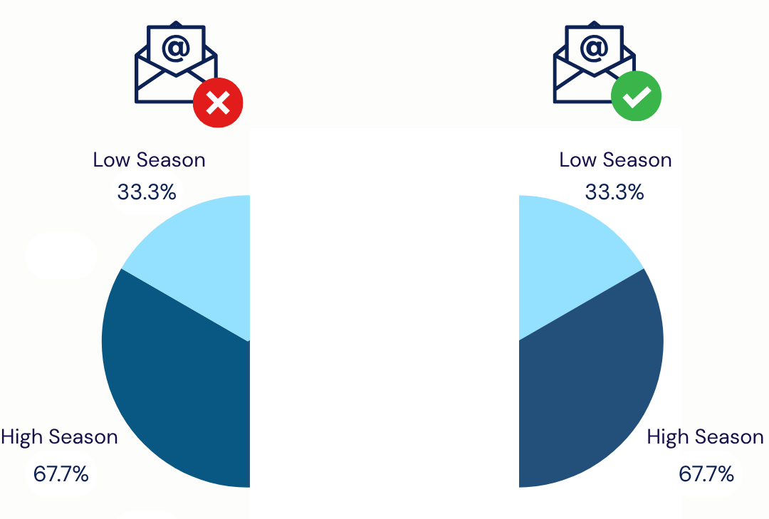
Because the treatment assignment probability is fixed at 0.5 for everyone, about 5,000 of the low-season customers will be assigned to treatment and about 5,000 to control. Likewise, about 10,000 of the high-season customers will be assigned to treatment and 10,000 to control.

As a result, the treated and untreated groups end up with the same distribution of seasonal conditions. In both groups, one third of the customers come from low-season conditions and two thirds from high-season conditions.

The only reason bias was produced by seasonality differences between the customers before was that the seasonal distribution differed between the treated and untreated units. Those differences in seasonal conditions produced differences in spending, and we could not attribute those differences to the effect of the treatment. But now, in the randomized case, customers in the treated and untreated groups are exposed to the same seasonal conditions on average. Because of this, any difference in average spending between the two groups can be attributed to the effect of the email. This makes it valid to write

ATE = E[Y | T = 1] − E[Y | T = 0].

Nevertheless, I can imagine that many people still feel confused at this point. It may feel counterintuitive that there is no consequence at all of the fact that many more customers in the experiment appear under high-season conditions than under low-season conditions. After all, if the experiment contains a much larger number of high-season customers, the data we analyse contain much more information from that part of the seasonal cycle. It is reasonable to wonder whether this should matter in some way.

And this is valid, because it actually can matter, not for bias, but for external validity.

To see this, note that the ATE we obtain reflects the mixture of seasonal conditions that happened to occur during the experiment. If two thirds of the customers appeared under high-season conditions, then two thirds of the information in the estimate comes from customers who were observed under those conditions. The remaining one third comes from customers in low-season conditions.

To see this more explicitly, note that the ATE can also be written as a weighted average of the treatment effects within each seasonal condition. In particular:

ATE = P(S = low season) × CATE(low season) + P(S = high season) × CATE(high season).

This identity holds because randomization ensures that treated and untreated units are comparable within each seasonal condition. The overall difference in average spending between the treated and untreated groups is therefore just equal to the difference within low-season units, weighted by how often low-season units appear, plus the difference within high-season units, weighted by how often high-season units appear.

In our example, if one third of the customers appear under low-season conditions and two thirds under high-season conditions, then:

ATE = (1/3) × CATE(low season) + (2/3) × CATE(high season).

This decomposition shows directly that high-season customers contribute more to the estimate simply because they occur more often in the experiment.

This becomes important when the effect of the email differs across seasonal conditions. If customers respond more strongly to the email during high-season conditions, then CATE(high season) will be larger than CATE(low season). In that case, an ATE that places most of its weight on high-season units will be larger than an ATE that places more weight on low-season units. This is not a problem for the experiment itself. The experiment estimates the correct causal effect for the mixture of seasonal conditions that happened to occur during the study window.

However, it may be a problem when we want to generalize the result. If we apply this ATE to a future period in which the seasonal composition is different, our ATE is probably wrong. For example, if the future period consists almost entirely of low-season conditions, and the effect is smaller in those conditions, then the effect for units in that future period will be lower than the effect estimated in the experiment. The difference arises because the treatment effect varies across seasonal conditions, and the seasonal composition has changed.

This is how seasonality can still matter, even when it does not produce bias. If the treatment effect differs across seasonal conditions, then the ATE we estimate is very sensitive to the mix of conditions present in the data. Since this mix can vary substantially over time, the ATE from one period does not necessarily apply to another period with a different seasonal composition, and this can strongly limit the generalizability of our analysis. In such cases, it might be better to focus on the conditional effects themselves and report the CATEs for the different seasonal conditions, rather than relying on a single ATE that is tied to a specific seasonal mix.

Finally, note that in many observational settings, seasonality does not take only one of the two roles we discussed. It can influence how likely a unit is to receive the treatment, and at the same time the treatment effect can differ across seasonal conditions. In these cases, both issues are present. The comparison of treated and untreated units is biased because the groups appear under different seasonal conditions, and an ATE estimate obtained after adjusting for seasonality may still have limited generalisability if the seasonal mix changes in the future. Also here, focusing on CATEs could be a better choice.

Conclusion

Seasonality influences how businesses operate, how customers behave, and how effective a treatment can be, which makes it one of the strongest forces present in most e-commerce settings. Because of this, it naturally finds its way into many causal analyses. Understanding the different roles it can play helps us interpret our results correctly and avoid drawing conclusions that do not hold outside the period we analysed. I hope this post has helped make that a bit clearer.