Demistifying the Exogeneity Assumption in Linear Regression

For many people in the data industry, Linear Regression is the first model they learn for data modelling. The focus then usually falls into one of two categories:

1. We aim to predict some variable Y as accurate as possible, and we use Linear Regression as a predictive model. In this case, we usually care about predictive accuracy, and focus on optimizing metrics like Mean Squared Error using techniques like Cross-Validation.

2. We aim to draw meaningful interpretations from the parameters of a Linear Regression model. In this case, we usually care about unbiasedness and the emphasis is on the exogeneity assumption.

The second case is very common, especially in YouTube videos, blog posts, and textbooks. Generally, these sources follow a similar structure. First, the form of the Linear Regression model and the Ordinary Least Squares (OLS) optimization method are introduced. Then, the Classic OLS assumptions are stated. One of these OLS assumptions then is the Exogeneity Assumption, which refers to mean-independence of the “true error” and the independent variables in the model. Then it is emphasized that this assumption is needed to ensure that our estimated Linear Regression coefficients are unbiased for the “true parameters” of the “true model” for outcome Y.

But unfortunately, this terminology is extremely ambiguous. What exactly is this “true model”? What are its “true parameters” and the “true error”? And why precisely does exogeneity ensure unbiasedness?

This ambiguity likely comes from the broader hesitation many people have when it comes to discussing causality. Sometimes it’s because the lecturers themselves are not properly educated on causality. Other times, it’s because bringing up causality can invite criticism, especially in an industry where association-focused analysis has long been the norm and causal claims are treated with caution.

But the reality is: exogeneity and unbiasedness only truly matter if we’re aiming to do Causal Inference with Linear Regression. The ‘meaningful interpretations’ we want to draw from the parameters in the model are causal interpetations. Without this purpose, the exogeneity assumption and unbiasedness loses most, if not all, of its importance.

In this blog post, I aim to clear up any confusion around the aformentioned terminologies. I’ll clearly explain what the “true model” of Y refers to, what the “true parameters” and “true error” actually mean, and how exogeneity ties into all of it.

The Linear Regression Model and its Parameters

Linear Regression is a statistical method used to model the relationship between variables. Typically, there’s one variable you aim to predict, called the dependent variable, and one or more variables you use to make predictions, called the independent variables. The idea is to model the dependent variable as a linear function of the independent variables, which is why it’s called Linear Regression.

Specifically, if Y is the dependent variable and X₁, X₂, … , Xₖ are the independent variables, Linear Regression models Y as:

Y = β₀ + β₁X₁ + β₂X₂ + ⋯ + βₖXₖ + ϵ

where k is the number of independent variables.

Here, β₀ is called the intercept. Generally, this intercept approximates E[Y | X₁ = 0, X₂ = 0, …, Xₖ = 0 ]. However, in many practical situations, it doesn’t have a meaningful interpretation. This is because it is often unrealistic or impossible for all the X variables to take on the value 0 (simultaneously). Imagine one variable representing something like the height of an individual: a height of 0 doesn’t make any sense. This often makes the intercept more of a mathematical component of the model rather than a meaningful quantity.

But this isn’t a problem, because the intercept generally isn’t our focus point if we are interested in interpreting parameters causally. Instead, the slope coefficients β₁, β₂, … , βₖ are.

These slope coefficients are what associate changes in some X variable with changes in Y. And Causal Inference is all about understanding how changes in one variable affect another. But the important thing here is to note the word “associate”. Slope coefficients in regression models are always just measures of (conditional) association, with no inherent causal meaning. More formally, a slope coefficient βⱼ in a multivariate regression model just discussed is computed as:

βⱼ = Cov(ϵₓⱼ , ϵᵧⱼ)/Var(ϵₓⱼ)

where ϵₓⱼ are the residuals obtained from regressing Xⱼ on all other X variables, and similarly, ϵᵧⱼ are the residuals obtaining from regressing Y on all other X variables except Xⱼ.

This is a fundamental result formalized in the Frisch-Waugh-Lovell Theorem, and it clearly shows that slope coefficients in Linear Regression models are just measures of association. A slope coefficient βⱼ just measures association between the part of Y not linearly explained by the other variables in the model (so except Xⱼ), and the part of Xⱼ not linearly explained by the other X variables in the model. In other words: it measures the association between Y and Xⱼ after partialling out the linear influence of the other variables in the model on their relationship.

So, Linear Regression parameters are always just measures of association. They do not have any inherent causal meaning, they don’t ‘prove’ causality. They are purely statistical, associational measures.

Nevertheless, they can be interpreted causally under certain conditions. When? Well, when association = causation. Sometimes, (conditional) associations between variables Xⱼ and Y only stem from a causal relationship between them. And when this happens is related (but not limited to) the exogeneity assumption often mentioned with Linear Regression. Let’s break this down.

The “True Model”

Exogeneity is generally used as an assumption that ensures our OLS coefficients are unbiased of the “true parameters” of the “true model” of Y.

So, what’s this true model? It’s a structural causal equation!

More specifically, define the structural causal equation for Y as

Y := θ₀ + θ₁X₁ + θ₂X₂ + ⋯ + θₖXₖ + e.

In this equation:

• X₁, X₂, … , Xₖ are the endogenous direct causes of Y.

• e represents all omitted causes of Y. Basically, it contains real variables just like X₁, X₂, … , Xₖ are, but which we either don’t observe, don’t measure, or choose not to include in the equation for whatever reason.

• “:=” emphasizes that this structural causal equation represents an assignment process: nature first determines on the values of X₁, X₂, … , Xₖ and only then assigns the value of Y as a linear function of the X variables. This is not a standard algebraic equation that we can rearrange to solve for one of the X variables in terms of Y.

• θ₁,θ₂, … , θₖ represent Controlled Direct Effects. That is, each causal parameter θⱼ represents the change in Y we would observe if we were to intervene on Xⱼ, increasing it by one unit, while holding all other X variables fixed through external intervention. So it quantifies the effect Xⱼ on Y that is not mediated by other variables in the system or, more accurately, the sensitivity of Y to changes in Xⱼ while all other factors in the analysis are held fixed.

Now, the exogeneity assumption isn’t needed for the parameters θ₁,θ₂, … , θₖ to have a causal meaning. In fact, it’s irrelevant to the meaning of these parameters. They always have a causal meaning, even if e is dependent on one or multiple of X₁, X₂, … , Xₖ. However, violations of exogeneity can affect our ability to estimate these causal parameters in an unbiased way using Linear Regression.

The Exogeneity Assumption

Even with the exogeneity assumption, educational sources are ambiguous. But the definition you’ll see most often is that exogeneity refers to mean-independence between e and the variables X₁, X₂, … , Xₖ:

E[e | X₁, X₂, … , Xₖ] = E[e]

Often this is further equated to 0 under the assumption that E[e] = 0, but this isn’t always necessary.

This assumption implies that knowing X₁, X₂, … , Xₖ doesn’t give us any additional systematic information about e compared to not knowing them.

The Implications of Exogeneity

When the exogeneity assumption holds, we have that β₁, β₂, … , βₖ in the (population-level) Linear Regression

Y = β₀ + β₁X₁ + β₂X₂ + ⋯ + βₖXₖ + ϵ

are equal to the respective θ₁,θ₂, … , θₖ in

Y := θ₀ + θ₁X₁ + θ₂X₂ + ⋯ + θₖXₖ + e

More specifically, if exogeneity holds, we have that β₁ = θ₁, β₂ = θ₂, …, βₖ = θₖ. In a sample-level Linear Regression, we have that each estimated βⱼ is an unbiased estimate for the respective causal parameter θⱼ.

In other words, under exogeneity, each parameter βⱼ can be interpreted as (an estimate of) the direct causal effect of a one unit increase in Xⱼ on Y.

I’ll break down why this is in a moment. But first, note here that the exogeneity assumption is applied to a structural causal error (e). So the “true error” is a structural causal error.

Sometimes, people refer to the true error as the error in a population regression, but this is wrong. An error in a population regression (which I’d refer to as a population residual) is just the difference between the fitted line and actual observed values of Y. It’s an artifact of imperfect model fitting with no real-world meaning. And actually, by construction of OLS, the population residual is always uncorrelated with the independent variables. That’s a mathematical fact, not an assumption. So it wouldn’t make sense to impose or emphasize a condition like exogeneity on something that’s already forced to be orthogonal to the independent variables.

A structural error is fundamentally different and contains real-world variables that cause Y. This can includes variables related to socioeconomic conditions, genetics or anything else. Exogeneity should be applied to a structural causal error!

Okay, so the “true model” is a structural causal equation, the “true error” is a structural causal error, and the “true parameters” are structural causal parameters (θ₁,θ₂, … , θₖ).

Now, why does exogeneity ensure that β₁ = θ₁, β₂ = θ₂, … , βₖ = θₖ?

Math

Let’s first show a simple mathematical explanation for this. It is well-known that Linear Regression approximates the Conditional Expectation Function (CEF). Specifically, the Linear Regression model

Y = β₀ + β₁X₁ + β₂X₂ + ⋯ + βₖXₖ + ϵ

approximates E[Y | X₁, X₂, …, Xₖ] as β₀ + β₁X₁ + β₂X₂ + ⋯ + βₖXₖ.

Now, a theorem called the Linear CEF Theorem states that if the CEF is linear, the population regression is it. In other words, if the CEF is linear, we have that E[Y | X₁, X₂, …, Xₖ] = β₀ + β₁X₁ + β₂X₂ + ⋯ + βₖXₖ.

Now, if Exogeneity holds, the CEF is linear. Because if we look at the structural equation for Y again:

Y := θ₀ + θ₁X₁ + θ₂X₂ + ⋯ + θₖXₖ + e

we have that

E[Y | X₁, X₂, …, Xₖ] = E[θ₀ + θ₁X₁ + θ₂X₂ + ⋯ + θₖXₖ + e | X₁, X₂, …, Xₖ]

= θ₀ + θ₁X₁ + θ₂X₂ + ⋯ + θₖXₖ + E[e | X₁, X₂, …, Xₖ]

= θ₀ + θ₁X₁ + θ₂X₂ + ⋯ + θₖXₖ + E[e].

Since E[e] is just a constant, the CEF is linear. Therefore, β₀ + β₁X₁ + β₂X₂ + ⋯ + βₖXₖ = θ₀ + θ₁X₁ + θ₂X₂ + ⋯ + θₖXₖ, and each regression parameter equals the respective causal parameter.

Okay, so that’s the math. What about intuition?

The Intuition Behind Exogeneity

Let’s focus on one parameter β₁. Why does E[e | X₁, X₂, … , Xₖ] = E[e] ensure that we have β₁ = θ₁?

Well, recall that in a Linear Regression Y = β₀ + β₁X₁ + β₂X₂ + ⋯ + βₖXₖ + ϵ, β₁ measures the association between the part of Y not linearly explained by X₂, X₃, … , Xₖ, and the part of X₁ not linearly explained by X₂, X₃, … , Xₖ. In other words, β₁ measures the association between X₁ and Y when holding X₂, X₃, … , Xₖ ‘fixed’. We often refer to this as that the model controls for X₂, X₃, … , Xₖ.

Now, if we look at the structural causal equation for Y again:

Y := θ₀ + θ₁X₁ + θ₂X₂ + ⋯ + θₖXₖ + e

We see that if we hold X₂, X₃, … , Xₖ fixed, any association left between X₁ and Y can only be produced in 2 ways.

First, we have that when X₁ has a direct causal effect on Y (θ₁ ≠ 0), then changing X₁ changes Y directly. This produces a causal association between them.

Second, we have that if e and X₁ are (mean-) dependent (conditional on X₂, X₃, … , Xₖ), then this produces a biased association between them. More specifically, if e changes, then Y changes, because e is a cause of Y. Now if e and X₁ are still (mean-) dependent after conditioning on X₂, X₃, … , Xₖ, this means that changes in e are also associated with changes in X₁. Therefore, changes in Y produced by changes in e will be associated with changes in X₁. This association is non-causal (bias).

This means that if e and X₁ are still (mean-) dependent after conditioning on X₂, X₃, … , Xₖ, the association measured by β₁ will (partly) be non-causal, which makes β₁ biased.

An important example why e and X₁ may still be (mean-) dependent after conditioning on X₂, X₃, … , Xₖ is that there is a variable in e that also causes X₁, whose influence isn’t blocked by conditioning on X₂, X₃, … , Xₖ.

To have that β₁= θ₁, we must have that β₁ only measures association coming from the direct causal effect of X₁ on Y, which happens if e and X₁ are independent conditional on X₂, X₃, … , Xₖ. And since E[e | X₁, X₂, … , Xₖ] = E[e] inherently implies that E[e | X₁, X₂, … , Xₖ] = E[e | X₂, … , Xₖ], exogeneity ensures that β₁= θ₁.

A similar reasoning applies to the other parameters.

Coding Example

Let’s code up an example to show everything discussed. This example comes from my course “Causal Inference with Linear Regression: A Modern Approach (Part I)”, and notation is slightly different than used in this blog post.

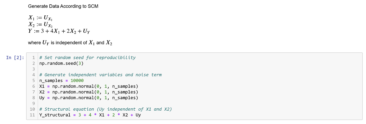
First, I generate data according to some structural equations, where X₁ and X₂ are just generated as their structural errors, and Y is generated as 3 + 4X₁ + 2X₂ + Uᵧ, where Uᵧ is the structural error of Y (this is e from before). Here Uᵧ is independent of X₁ and X₂. Since general independence implies mean-independence, we have that the exogeneity condition

E[Uᵧ | X₁, X₂] = E[Uᵧ]

holds. Therefore, running a Linear Regression of Y on X₁ and X₂ should result in unbiased parameter estimates that can be interpreted causally.

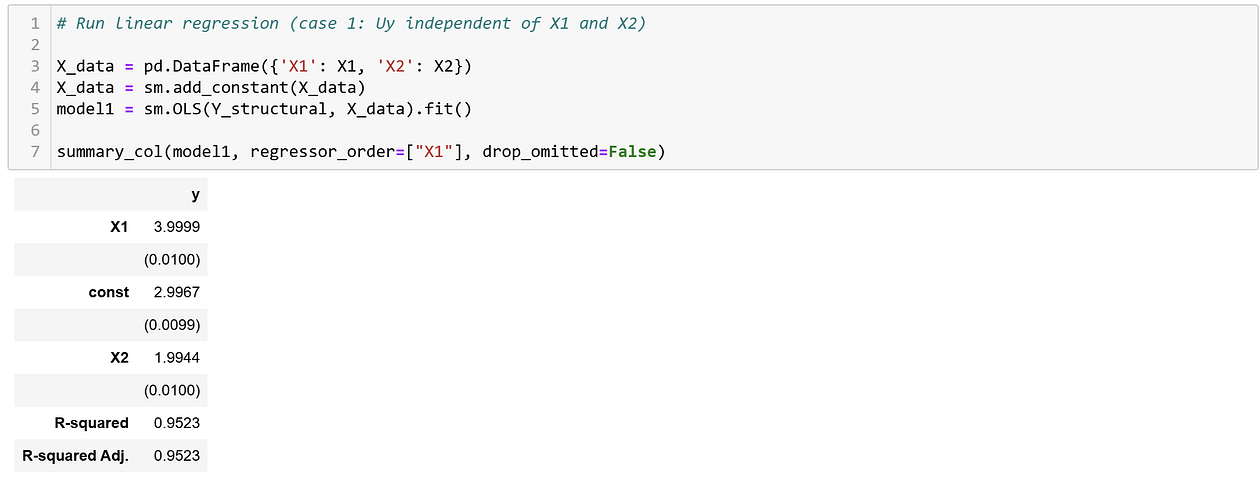
Indeed, the coefficient for X₁ is 3.999, while the true causal parameter was 4, and the coefficient for X₂ is 1.9944, while the true causal parameter was 2. Any differences are due to the fact that we work with a sample and not with an infinite population.

Next, let’s violate the exogeneity condition and see what happens.

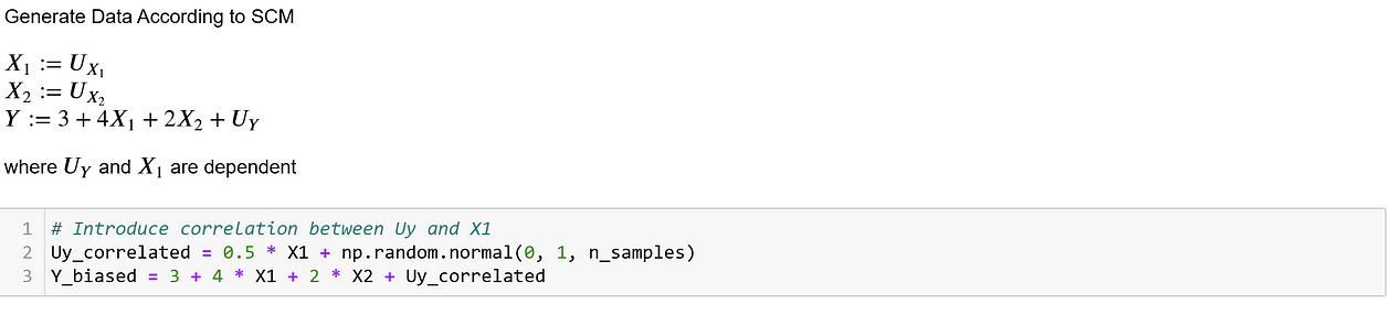
Specifically, I adjust the data generating process to now have a dependence between structural error Uᵧ and X₁. In this case, we have that

E[Uᵧ | X₁, X₂] != E[Uᵧ],

since, conditional on X₂, X₁ still provides additional information about Uᵧ. If I now run the same regression as before, I get the following results.

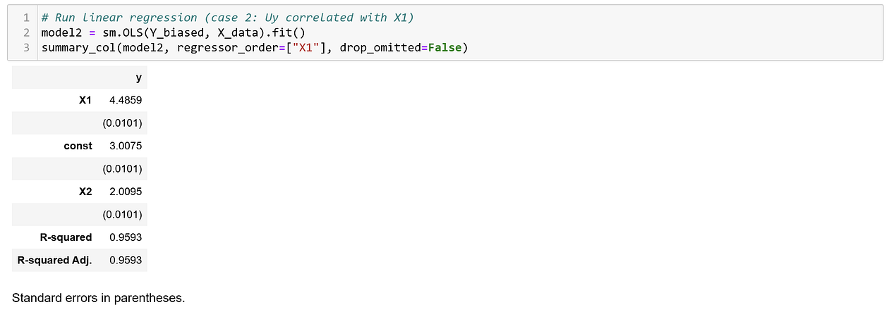
The coefficient for X₁ is now 4.4859, while the true causal parameter of interest is 4. To demonstrate that this difference is not due to limited sample size, I generated 1,000,000 samples from the same data generating process, and ran the regression again.

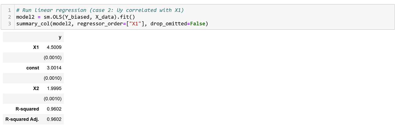
The coefficient is 4.5009, which is clearly different from 4. So, violations of exogeneity made our estimated β₁ biased.

That said, if we look at the coefficient for X₂, we see that this coefficient is actually still unbiased. This shows something important: while exogeneity is sufficient to ensure all coefficients have causal meaning, it’s not necessary if we only want one or a few coefficients to have causal meaning.

Relaxing Exogeneity

With Causal Inference in practice, we usually just want to know the effect of some treatment variable on an outcome. This means that if we’d use Linear Regression for this purpose, our main focus is that the treatment coefficient(s) are unbiased, the other coefficients don’t really matter.

In such cases, the traditional exogeneity can be relaxed, and we also do not necessarily have to run a regression of Y only on its direct causes. Instead, we just need to add variables that de-bias our treatment coefficient of interest. If I relate this back to the structural error e again, what we need is that any dependence between e and the treatment variable of interest should be blocked out by the other variables we include in the model.

To understand which variables are sufficient for this purpose, we can make use of Causal Directed Acyclic Graphs and Graph Criteria (Judea Pearl’s Structural Causal Model Framework).

Conclusions and Recommendations

Hopefully, this blog post helped clear up some of the causal confusion that often comes with traditional education on Linear Regression. But there’s still much, much more to say about how Linear Regression works for Causal Inference. In fact, it’s one of the most fundamental models in the entire field.

Because I think this foundation is so important (and underrated), I’ve created a full 2-part course series on the topic. Feel free to check them out in the courses section of the Causal Academy.