Coping with Causal Graph uncertainty in Causal Inference

The concept of Causal Graphs, introduced by Judea Pearl, has significantly advanced the general understanding of Causality in the data industry. When we are interested to estimate the causal effect of some variable T on an outcome Y, Causal Graphs are an intuitive tool we can use to understand what biases may exist in their relationship, and how we can remove them. But these Causal Graphs aren’t given to us: they must be created by us. This comes with inherent uncertainty. In this blog posts, I want to talk a bit about this uncertainty, and main strategies we can use to cope with it.

How We Use Causal Graphs

With Causal Inference in practice, we are often interested to estimate the causal effect of one variable on another. This means we are interested in aspects of the data generating process (DGP). Ideally, we would like to take control over this DGP, change the value of one variable and observe how this changes another variable. But ofcourse, this is not possible in reality.

When we perform Causal Inference with observational data, all we have are realizations of joint distribution of variables. And these joint distributions are often not unique to one DGP. Instead, multiple DGP’s can produce the same joint distribution. This means that observational data alone can never reveal the underlying DGP.

All we can do with our observational data is observe and model associations. But although these associations can partly be produced by a cause and effect relationship between the variables of interest, they are generally biased. This means that part of the association is non-causal in nature, for example because the variables have a common cause. To estimate causal effects with observational data, we somehow need to remove this biased part in the associations.

And the first step to do this is to understand in what way these associations are biased. Again, observational data will not reveal this to us. We must add external knowledge to our observational data. Specifically, we must make assumptions about the process that generated our data.

Causal Graphs, or more formally, Causal Directed Acyclic Graphs, are a means to clearly represent our assumptions about the data generating process.

For example, say we are interested in the causal effect of owning an electric vehicle (EV) on annual miles driven. We might have data on whether individuals own an EV or not, their annual miles driven and various characteristics. We can use this to compute for example the average annual miles for EV owners and non-EV owners and compare them. But since association is not causation, this difference likely doesn’t reflect the causal effect that owning an EV has on annual miles driven.

To gain more clarity about what biases might exist, we may draw a Causal Graph like this:

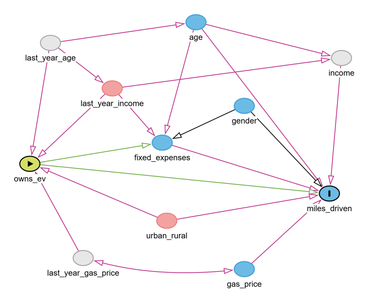
Edges with 1 arrow head indicate that we suspect that the start node might causally affect the other node directly. In other words, if all other variables are held fixed, and we’d change the starting node, then it could possibly change the distribution of the end node. Edges between two variables with 2 arrow heads indicate the presence of an unobserved common cause between these variables.

Using this Causal Graph, we can understand what biases exist in the relationship between owning an EV and annual miles driven. I won’t go deep into this in this blog post, but in summary:

• We look for all paths that connect the variables of interest. These paths can be either causal or non-causal, and produce certain association flows along them.

• We can condition on variables to block or open certain association flows.

• We then look for variables that block all non-causal paths, and keep open all causal ones. This is done using Graph Criteria like the backdoor criterion. This results in an adjustment set of variables such that, when we condition on them, remove all bias between the variables of interest.

• We then have that association = causation, and we can use regular predictive modelling techniques and observational data to estimate the causal effect of interest.

(If you want to learn more about this, check out the courses on Causal Academy).

The Inherent Uncertainty With Causal Graphs

If our Causal Graph is correct, then any adjustment set of variables found using criteria such as the backdoor criterion is sufficient. In other words, if we properly adjust for these variables, we can use observational data and association-based methods to estimate the causal effect we’re interested in.

But here’s the problem: a Causal Graph isn’t something that’s given to us. In practice, we have to build it ourselves. And that comes with uncertainty, because what if the graph we’ve drawn doesn’t accurately reflect the true process that generated the data?

To put this into perspective, consider that with just 7 nodes, there are 1,138,779,265 possible Causal DAG’s. What are the chances that the one we picked is the correct one? Probably not very high…

So, what are the consequences if our Causal Graph is incorrect?

Well, if our Causal Graph is incorrect, then a ‘sufficient’ adjustment set found might not actually be sufficient. This means that if we adjust for these variables in our modelling process, we might think our estimate is based purely on causal associations, but in reality, it’s still based on biased associations (though maybe less biased than before). This means we will either overestimate or underestimate the true causal effect of interest. How problematic this is depends on the extent that bias is still present, and the specific problem we’re aiming to solve.

Now, I don’t want to sound too negative, but the truth is, we can never fully validate a causal graph. There is no technique we can use that will give us an answer like “Yes, this perfectly represents the true data-generating process.”

That’s just the reality, but it shouldn’t discourage us. Even though we can’t prove a Causal Graph is correct, there are methods that help us build a reasonably accurate one. Let’s go over some of the most important ones.

Domain Expertise

First things first, we need to talk about what is essential for creating and adjusting a Causal Graph. At the core of the entire process is domain expertise. This refers to knowledge specific to the problem we are studying. It can come from people with deep experience in the field or from prior research and literature.

In traditional predictive modelling, data science teams can often work somewhat independently from domain experts because the data itself drives most of the modelling decisions. But with Causal Inference, that is not the case. The modelling process is guided by external knowledge, not just the data.

Sometimes, experienced data scientists have enough background to act as domain experts themselves. But that is not a requirement. Causal Graphs can be developed in teams that include domain experts without any data modelling experience. What matters is that they can help us think through the kinds of causal relationships that are likely to exist in their area of expertise and that might be relevant to the problem we are trying to model.

To reduce subjectivity and strengthen the graph, it is best to work with multiple domain experts when possible, and to combine their input with evidence from the literature.

Time

There’s another concept that is incredibly helpful for building an accurate Causal Graph: time.

While most parts of constructing a Causal Graph involve uncertainty, time gives us something to hold on to. Because one thing we do know for sure is that causes must come before their effects. Something in the future can’t cause something in the past. This logical understanding can be surprisingly powerful. When you’re feeling stuck or unsure while building a Causal Graph, returning to the concept of time can really help, because it often narrows down the number of plausible Graphs a lot.

Personally, when I’m unsure about whether there should be an edge from node A to node B, I ask myself:

“If I could intervene on node A, and suddenly enforce a different value across an entire population, do I deem it possible that I would see a change in B (when all other variables are held fixed)?”

If the answer is yes, I draw an edge. The idea of intervention is closely linked to the idea of time: if we intervene on something now or in the future, it can never affect something that has already happened.

Okay, so those are some useful practices for building a Causal Graph. But now the question is: how can we become more confident that the graph we’ve built is a reasonable representation? The first data-driven technique we can use is conditional independence testing.

Conditional Independence Tests

We can’t prove the correctness of Causal Graphs, but we can falsify them. More specifically, our approach to building an accurate Causal Graph is about actively searching for evidence that shows us our model is wrong. When we find it, we reject our model, build a better one, and repeat. So basically, in practice, your goal is not getting the true Causal Graph, but getting a hard-to-reject Causal Graph.

Conditional independence tests are one of the most important tools we can use to falsify a Causal Graph. Why? Well, causal relationships constrain the data in certain ways, one of which is by forcing variables to be conditionally independent.

Take this example. A child’s eye color is determined by the genes they inherit from their parents. The parents’ genes, in turn, are inherited from their parents — the child’s grandparents. So the structure looks like this:

eye color genes of grandparents → eye color genes of parents → eye color of child

This setup creates a general dependence between the genes of the grandparents and the eye color of the child. Certain combinations of grandparent genes can make some parent gene combinations more likely, which in turn affects the child’s eye color. But once we know the genetic makeup of the parents, the grandparents’ genes no longer provide extra information: the child’s eye color becomes conditionally independent of the grandparents’ genes, given the genes of the parents.

This kind of conditional independence is implied by the Causal Graph. If the graph is correct, we should see this independence in the data. That’s something we can test with statistical tools. And if the data shows a strong dependence where the graph says there should be independence, then the graph is wrong.

This logic is formalized using the concept of d-separation. If two variables, X and Y, are d-separated by a set of variables Z in the graph, then X and Y should be conditionally independent given Z in the data. If they’re not, we reject the graph and go back to revise it. We repeat this process until we arrive at a graph that we can no longer reject based on the data.

Conditional Independence Tests (Latent Variables)

Not all independence tests implied by our Causal Graph can actually be tested with the data. This is because Causal Graphs often include variables that are not in our dataset. That is not a problem with the graph, it’s just the nature of what we are trying to do. Causal Graphs aim to represent the data-generating process, not just the data we happen to observe. And the true DGP does not care what is or is not in your dataset.

As a result, your Causal Graph will likely include unobserved variables, which we call latent variables. Any conditional independence tests that involve these latent variables cannot be performed, simply because we do not have data on them.

But even when a latent variable is unobserved and prevents us from testing standard conditional independencies, it can still leave behind a detectable footprint. Specifically, certain graph structures that involve latent variables can imply algebraic constraints among the observed variables. For example, they can create independence relationships between observed variables and functions of other observed variables.

These types of constraints are known as Verma Constraints.

In this way, Verma Constraints provide an indirect way of testing and potentially falsifying Causal Graphs, even when they involve latent variables.

An important consideration when using statistical tests is that statistical independence is not the same as true independence. We might conclude that two variables are dependent based on a statistical test, even if they are actually independent, or the other way around. This is simply a limitation of working with imperfect, finite data and probabilistic inference.

Additionally, the more statistical tests you perform, the higher the chance of making errors (a well-known issue called the multiple comparisons problem). This means that with enough tests, some results will appear significant just by chance.

Because of this, it’s important to prevent yourself of becoming overly focused and reliant on the outcome of conditional independence tests alone.

Causal Discovery Algorithms

So far, we have focused on building Causal Graphs using domain knowledge and the concept of time, and then trying to falsify them with data through conditional independence tests. But there is another category of tools that I think sits somewhere in between these two steps: Causal Discovery Algorithms.

Causal Discovery Algorithms aim to learn Causal Graphs directly from the data. There are several types of approaches.

Constraint-based algorithms work by essentially reversing the conditional independence logic we just discussed. They analyze which conditional independencies exist in the data and then limit the possible Causal Graphs to only those that are consistent with those patterns.

Score-based algorithms take a different approach. They search for Causal Graphs that receive high scores based on how well they fit the data according to some scoring function.

Function-based algorithms assume a specific functional relationship (like linear or non-linear equations) between variables. These methods use certain asymmetries created by these functional forms to help identify the direction of causality.

Continuous optimization-based algorithms treat the search for a Causal Graph as a continuous optimization problem, where the goal is to find the graph structure that best explains the data under certain constraints.

In most of these methods, prior knowledge can also be incorporated. For example, you can specify which edges must or must not be present, or introduce Bayesian priors over the graph structure to guide the learning process.

So basically, these algorithms can help us come up with a Causal Graph directly from the data. And at first glance, Causal Discovery Algorithms sound like a holy grail to most people. This is because it aligns well with what we are comfortable with and used to in the data industry: to let the data speak.

But there are important caveats.

These algorithms often rely on strong assumptions that can’t be tested, and they are often very sensitive to latent variables. As discussed earlier, Causal Graphs aim to model the DGP, not just the variables in the dataset. However, Causal Discovery methods generally only use the variables that are present in the data. If an important variable (such as a common cause) is missing, the algorithms can create edges between variables that aren’t actually causally connected. Some algorithms have ways to cope with this, but others don’t.

That is why I do not see Causal Discovery Algorithms as the leading tool to use when creating a Causal Graph. And they are not really meant for falsifying graphs either. Instead, I think they are best thought of as supporting tools: something to help us think more broadly, question our assumptions, and avoid tunnel vision.

We can use them to generate hypotheses and then compare the results with what we believe makes sense. If the discovered structure aligns well with our expectations, it can increase our confidence that our assumptions are consistent with the data. If it does not, that is an opportunity to rethink our Causal Graph (to look at which edges are different from our hypothesized graph, and ask whether those relationships are plausible).

In the end, these algorithms are another tool to help us build better Causal Graphs. Not by blindly accepting their output, but by using them to get new perspectives and continue questioning our assumptions.

Sensitivity Analysis

Sensitivity Analysis is an indirect, but powerful way to deal with uncertainty in our Causal Graph. Rather than focusing on the graph itself, it focuses on how misspecifications in our Causal Graph would affect our causal effect estimate.

Specifically, after performing the aformentioned procedure to come up with an as robust Causal Graph as possible, we’ll use this Causal Graph to identify a sufficient adjustment set: A set of variables such that when we adjust for them properly, we obtain an unbiased causal effect estimate. But although we did our best to make the graph as good as possible, it’s likely still wrong. So, what if our graph is missing something important? For example, what if there is a common cause of two variables that we didn’t include? If such a variable exists, adjusting for it would change the estimated effect. But by how much?

This is exactly where Sensitivity Analysis comes in. It helps us understand how much our causal effect estimate would change under different assumptions about the strength of missing variables (typically unobserved common causes, also called confounders). It does not tell us whether such variables actually exists, or how strong they really are. Instead, it shows us how our causal effect estimate would behave if omitted confounders of various strengths would exist.

Then, it’s up to us to reason about how realistic it is that ‘problematic’ omitted variables actually exist. For example, if the analysis shows that only extremely strong confounders would meaningfully change the estimate, we can be more confident in our conclusions. Because then it’s unlikely a confounder exists that would change our conclusions.

So, sensitivity analysis does not try to confirm whether our Causal Graph is or isn’t correct. Instead, it starts from the assumption that the graph is not entirely correct (which is usually the case in practice), and reasons about the impact these misspecifications may have on our results.

And it is not limited to issues with the Causal Graph alone. Sensitivity Analysis can also help when there is uncertainty about how we adjusted for variables. Even if we included the right variables, what if we adjusted for them incorrectly? For example, what if a variable influences the outcome in a non-linear way, but we only adjusted for it linearly? In many cases, Sensitivity Analysis can help us understand the impact of that kind of functional form misspecification too.

This is what makes Sensitivity Analysis one of the most important tools for dealing with uncertainty in Causal Analysis.

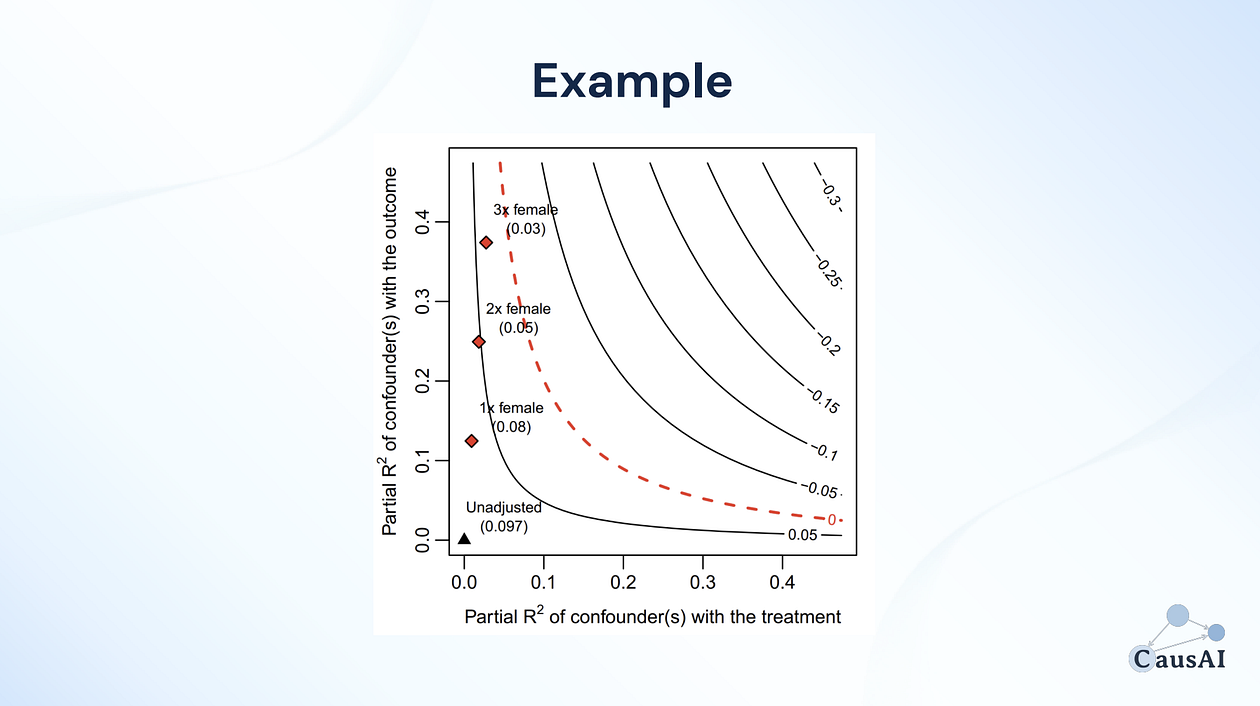
Slide from the course “Causal Inference with Linear Regression: A Modern Approach (Part I)".

Considerations

As you’ve seen, constructing a reasonable Causal Graph is a task of its own, and there are several techniques and tools that can support this process. Beyond the main approaches discussed here, there are even more methods available. But in the end, it’s important to remember that these tools are there to help us build the most accurate graph we reasonably can, not a perfect one.

It’s okay if our Causal Graph isn’t perfectly correct. What matters is that it’s not problematically incorrect in the parts that affect our analysis. In practice, only specific parts of the graph will actually play a role in our causal analysis. So even if some implied independence conditions fail in areas of the graph that aren’t relevant to the causal effect we’re studying, it’s usually not a major issue.